Kelly Criterion In Practice Part 1

A friend of mine recently forwarded an article by Kyle Mowery of GrizzlyRock Capital where he discusses the Kelly Criterion and how his fund implements it for position sizing. First off, I'll say kudos to GrizzyRock Capital for a thoughtful approach to position sizing. I've written numerous times about the benefits and deficiencies of the Kelly Criterion and Mr. Mowery's article does a good job of laying out the implementation and some of the benefits and detriments of Kelly. I'd like to use Mr. Mowery's article as an opportunity to discuss some of the benefits of a disciplined approach to position sizing while discussing some of the limitations of Kelly.
‍

Mr. Mowery correctly highlights that his fund's use of Kelly helps increase portfolio potential returns and reduce behavioral bias. The later aspect of behavioral bias is the benefit I find to be the most important attribute of adopting a process for sizing positions. Basic questions like, "how much can we make, what is the downside risk, and what are the probabilities of each", must be answered before any asset is placed in the portfolio. These questions are imperative to the fund's success and can be overlooked or poorly accounted for if not required as an input to the model. Potentially flawed position sizing derived by instinct and heuristics are highlighted by an optimal position size. Granted there may be legitimate reasons to have a position size other than the suggested optimal, but at least with a model, the difference is highlighted and justified.

Equal weighting is a model that many firms employ to counter the effects of behavioral bias. Mr. Mowery discusses the pros and cons:
‍

Some allocators elect to equal-weight investments given uncertainty regarding which investments will perform best. This strategy creates a basket of attractive investments that should profit regardless of which investments in the basket succeed. This method benefits from simplicity and recognizes the future is inherently uncertain. Drawbacks of the strategy include underweighting exceptional investments and overweighting marginal ideas.

I would add that equal weighting suffers also from the cliff effect and static rebalancing. The cliff effect is simply that the best idea and the 20^th best idea all get 5% exposure then the 21^st best gets 0%. That drop off the cliff is clearly suboptimal. Second, equal weighting is static in that it either rebalances positions back to equal weight as prices change or it lets them ride. Either way, the impact of falling risk/reward as prices rise is not accounted for until the position goes from equal weight to 0%. Trading around positions is a huge benefit of a position sizing model that can add large amounts of alpha. Equal weighting simply misses much of the trading benefit.

Mr. Mowery goes on to discuss allocating capital to ideas with the most potential:
‍

Another strategy is to allocate large amounts of capital to the investment ideas with the most potential. This methodology suggests investors should invest proportionally according to their ex-ante return expectations. The advantage of this methodology is matching prospective return to investment size. However, this strategy breaks down when allocators are incorrect about future investment return or risk prospects.

I'm not sure here if Mr. Mowery is talking about the return to the upside case or an expected return which is probability-weighted and includes downside. Either way, the argument against this method, "this strategy breaks down when allocators are incorrect about future investment return or risk prospects" isn't a successful counterpoint for why Kelly is better because Kelly will also be wrong if the inputs are wrong.

Kelly Formula Based Position Sizing. The Kelly Formula is great, but it is my belief that the Kelly Formula is sub-optimal to expected return-based sizing for portfolio management because it assumes that 100% of the bankroll can be bet on any one investment and it requires bimodal inputs (upside and downside only). Kelly's base assumption that 100% of capital can be allocated to a single bet necessitates that the formula is naturally cautious when sizing a position that has potential loss. It is my belief that expected return based position sizing (controlled for distribution width) is superior to Kelly.

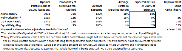
I recently ran a Monte Carlo simulation comparing the Alpha Theory position sizing technique to a myriad of common position sizing methodologies including Kelly Criterion (Optimal F), Up / Down Ratio, Equal Weighting (and by proxy 14 Markowitz Mean-Variance Modern Portfolio Theory systems - Two studies of Markowitz Mean-Variance systems show that mean-variance maximization does not beat Equal Weighting (DeMiguel et al (2006) / Jobson-Korkie)).  Alpha Theory measured success by measuring the amount of Portfolio Expected Return added per 1% of portfolio exposure.  Alpha Theory beat the closest methodology, Kelly Criterion, by 18%, Up / Down Ratio by 52%, Equal Weighting by 48%.

Kelly Criterion is the superior method for generating the maximum long-term geometric expected return when the whole portfolio can be wagered on a single investment.  However, portfolios are comprised of multiple investments and thus Kelly Criterion under bets good expected returns because it's trying to protect against complete loss of capital and over bets poor expected returns with very high probability of success.  Because portfolio investing has inherent capital protectors by limiting position size maximums, Kelly Criterion breaks down.
‍

-To prove this out I performed a Monte Carlo simulation which randomly created 10,000 portfolios of 50 stocks

-Randomly assumed that analyst's upside, downside, and probability estimates were up to 50% inaccurate

-Random variables included: assets, scenarios, success/failure of analysis, and position size and expected return parameters

-Alpha Theory (Expected Return adjusted for distribution width) created the optimal portfolio 7,074 times out of 10,000 (71%)

-Alpha Theory was 53% better than the next best method, Kelly Criterion
‍

Kelly Maximization of Long-Term Geometric Expected Return. I have seen several workarounds that use the Kelly Formula to construct a portfolio but most focus too heavily on the bet size of each individual investment. If John Kelly were alive today, I imagine he would probably tell us that the formula is a shortcut and the more important concept is finding the portfolio that maximizes long-term geometric expected return. That was the assumption that I made when I constructed my own Kelly calculator. The first step was scrapping the Kelly Formula and coming up with a way to account for investments with multiple scenarios and loss less than 100%. I could not figure out a way to make a closed-form solution, which is one of the best attributes of the Kelly Formula. I had to create an open-form calculator that used an iterative formula using the Solver function in Excel (there is a similar calculator at http://www.albionresearch.com/kelly/). With my new calculator I could create any investment with various economic outcomes and probabilities and derive the bet size that would give me the maximum expected return over the long-term (geometric). I made an assumption that I could not bet more than 100% (-100% for shorts). In reality, a fund could leverage investments and receive higher returns but for this portfolio example I assumed no leverage.

Trial #1. I plotted out the Kelly bet for a bunch of random investments and noticed the Kelly bet did not match up with the position size I would have expected for the portfolio. This is because the Kelly bet was not considering the portfolio. However, I did find that expected return was a good predictor of portfolio position size (example below).

We have 3 potential investments with which to build our portfolio. If I look simply at the Kelly Bet, I would maximize Investment #1 and #2 because they are 100% versus 80% for Investment #3. But the Expected Return for Investment #3 is higher than #1 and #2. This is the point where I hypothesized that I could compute the Maximum CAGR (Compound Annual Growth Rate) by investing the Kelly Bet of each investment, calculating the CAGR (14%,15%,16%), and then use the CAGR as a way to determine the correct position size. This certainly seemed to point in the right direction but it still did not feel right to have them so closely sized. I decided that the ultimate method would be to skip the calculation of individual bets and calculate which bets would maximize the expected return of the portfolio (Uncorrelated Portfolio bet size in chart). As you can see, to maximize the portfolio's return, the best allocation was to bet 43% on Investment #1, 6% on Investment #2, and 51% on Investment #3. This array of bets is how I came to the conclusion that the original Expected Return was a great predictor of portfolio position size.
‍

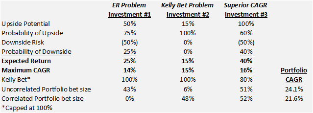
Correlation in Trial #1. But then I thought about the Central Limit Theorem and I realized that diversification makes a difference when assets are uncorrelated. But what if they are correlated? The benefit surely must be reduced. I subsequently built a string of payoffs where the gains and losses of Investment #1 and #3 occur in the same period (#2 doesn't matter because it always goes up 15%). When I recalculated the Correlated Portfolio position sizes, I got 0%, 48%, 52%. No exposure to Investment #1 in the Correlated Portfolio when the Uncorrelated Portfolio suggested a 43% position size.

This tells me that the correlation inside the array of outcomes has a large bearing on position size. What I needed to do is ensure that each array properly matches the inter-correlation amongst assets in the portfolio. At this point, I'm still working on that issue but maybe a starting point is the historical correlation and beta of each asset to the portfolio and other assets. Next, build thousands of hypothetical arrays of returns for each asset based on the scenario analysis. Finally, pick the set of hypothetical arrays that is most closely aligned with the inter-correlation of assets. From there we can iterate position sizes or use an optimization function that finds the portfolio with the maximum CAGR.

Speaking of maximum CAGR, see how both portfolios have higher Portfolio CAGR (24.1% and 21.6%) than any of the individual investments (14%, 15%, 16%)? This is the benefit of portfolio construction, which in this case is 5 to 10% of return.

Check back tomorrow for the 2^nd Trial and conclusion.