Kelly Criterion In Practice Part 2

As a continuation to Kelly Criterion in Practice Part 1 we dive into more tests and conclusion of the evaluation of the Kelly Criterion for portfolio management.
‍

Trial #2. The performance improvement of the portfolio made me wonder how a group of investments with similar Expected Returns (all 20%) but different payoff structures would look (see below).
‍

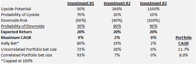
Here we see that neither the Uncorrelated or Correlated portfolio includes Investment #3 because it is severely impacted by its 90% chance of complete loss even though its expected return is 20% like the others. Investment #1 is favored by a wide margin because it has the lowest probability adjusted chance for loss of 15% (50% loss * 30% probability) versus 32% for Investment #2 (40% loss * 80% probability) versus 90% for Investment #3 (100% loss * 90% probability). In this case, the Kelly bet did a very good job of constructing the portfolio. This makes sense because the problem with the Kelly Formula for portfolio management is that it looks at each bet individually. We allowed the Kelly Formula to work individually by making all of the investments have the same Expected Return of 20%.

One of the most interesting outcomes of the second portfolio trial is that the CAGR of the Correlated Portfolio is 8.0%. That is lower than the 9% attained we could get from just betting the Kelly Bet of 80% in Investment #1 and holding the other 20% in cash. In this case, the best result is not a portfolio. I believe this is an important caveat in portfolio construction and should make cash an option for any portfolio. So instead of 3 Investments, you would always have 4 because cash may be a better option in certain circumstances.

Lessons Learned. So what have we learned from this analysis:

-Kelly bet size alone is not sufficient to determine position size

-Expected Return alone is not sufficient to determine position size

-Investment correlation has a large bearing on position size

-Probability Adjusted Chance for Loss has a large bearing on position size (Probability * Potential Loss)

-Cash is a legitimate option even if it has a 0% expected return

Ultimate Solution. The ultimate solution requires incorporation of research's scenarios analysis, correlation amongst assets, and picking the array of position sizes that maximizes long-term geometric expected return. The first step is to forecast thousands of arrays of returns for each investment based on its probability weighted scenario analysis resulting from your analyst's research. Next, choose the one set of arrays from the thousands generated which most closely matches the correlation statistics for each asset and the portfolio. Finally, use the best set of arrays to interpolate the bet size for each investment that maximizes portfolio return (if someone knows of a closed-form way of producing the array of position sizes please let me know).

Problems with the Ultimate Solution.

-Forecasting payout streams that have inter-correlation is very difficult. They could be calculated with historical correlations but that would suggest that future correlations will be the same as the past. The firm could forecast correlations but that is complicated and may be too much to ask from an operational perspective.

-The arrays are constructed at random which causes them to change with each iteration. This could cause unnerving degrees of variance in optimal position sizes depending on the randomized set of arrays. For instance, you could see that the optimal position size for IBM is 4.3% one minute, have nothing change, and the optimal position size move to 4.6% because the random array being selected has changed. My guess is the arrays would have to be stabilized until the addition of a new asset or research is updated. There is some work being performed by Sam Savage to standardize arrays.

-An optimization function is required to incorporate time horizon, liquidity, gross and net exposure, sector exposure, analysis confidence, etc. Certainly not an insurmountable hurdle, but could pose pitfalls.

Conclusion. Alpha Theory has tackled the problem in a straightforward way that accomplishes much of the task of position sizing described above. As we showed in Trial #1, Expected Return is a good predictor of position size in situations where there is variance in Expected Return. The predictive power is greatly enhanced by adjusting for the probability-weighted chance for loss (loss * probability of loss) which Alpha Theory does. The result is position sizing that is close to optimal position sizing (non-correlated). Lastly, because Alpha Theory is a linear function, it gives stable results and can scale position size to control for minimum and maximum position size, return parameters, liquidity, market correlation, time horizon, sector exposure, portfolio exposure, etc. Alpha Theory represents the best solution by providing most of the benefits of the complex ideal while still maintaining practicality for everyday use. At a bare minimum, it is light-years ahead of what most money managers are doing today!