Understanding Kelly For Portfolio Management

"It is my view that very few managers spend any time attempting to define the appropriate sizing of positions to mitigate downside and maximize returns."
– Peter M. Lupoff, Tiburon Capital

‍

I've spent the last 5 years helping firms develop better ways to construct portfolios of investments. On my journey I've come across portfolio managers espousing the superiority of the Kelly Formula for position sizing which was popularized by William Poundstone in his book "Fortune's Formula.". In concept, Kelly sounds like a good plan because it is a system that maximizes the long-term geometric return of a gambler's bankroll. The formula is:

where:

• f* is the fraction of the current bankroll to wager;
• b is the net odds received on the wager (that is, odds are usually quoted as "b to 1")
• p is the probability of winning;
• q is the probability of losing, which is 1 − p.

As an example, if a gamble has a 60% chance of winning (p = 0.60, q = 0.40), but the gambler receives 1-to-1 odds on a winning bet (b = 1), then the gambler should bet 20% of the bankroll at each opportunity (f* = 0.20), in order to maximize the long-run growth rate of the bankroll.

Source: Wikipedia

Kelly pros and cons. Bets are like investments in the sense that they both have probabilistic expectations of economic gains and losses, but betting assumes a possibility of deploying your entire capital (bankroll) to a single bet. However, investors construct portfolios where no single investment would consume the entirity of the firm's capital. So, the Kelly formula is not designed for portfolio management because it ends up under-weighting good expected returns and over-weighting poor expected returns. The Kelly logic is designed to avoid bankruptcy when betting the entire bankroll is an option. Investors inherently protect against catastrophic events by limiting the maximum position size of any one investment. This alone greatly reduces the predictive power of the Kelly Formula for portfolio management. An additional knock against the Kelly Formula is that it assumes a loss is always 100% of the bet but most equity investments have losses smaller than 100%.

I have seen several workarounds that use the Kelly Formula to construct a portfolio but most focus too heavily on the bet size of each individual investment. If John Kelly were alive today, I imagine he would probably tell us that the formula is really just a shortcut. The more important concept is to find the portfolio that maximizes long-term geometric expected return. That was the assumption that I made when I constructed my own Kelly calculator. The first step was scrapping the Kelly Formula and coming up with a way to account for portfolios with maximum position sizes, investments with multiple scenarios and losses less than 100%. I'm not a mathmetician, so a closed-form solution to the problem was out of my reach. In closed-from, I put in some variables and it gives me a result, which is one of the best attributes of the Kelly Formula. I had to create an open-form calculator that used an iterative formula using the Solver function in Excel (there is a similar calculator at http://www.cisiova.com/betsizing.asp). With my new calculator I could create any investment with various economic outcomes and probabilities and derive the bet size that would give me the maximum expected return over the long-term (geometric). I made an assumption that I could not bet more than 100% (-100%for shorts). In reality, a fund could leverage investments and receive higher returns but for this portfolio example I assumed no leverage.

Trial #1. I plotted out the Kelly Formula bet (original formula from the beginning of this article) for a bunch of random investments and noticed the Kelly bet did not match up with the position size I would have expected for the portfolio. This is because the Kelly bet was not considering the overall portfolio. However, not surprisingly, I did find that expected return was a good predictor of optimal portfolio position size (example below).

We have 3 potential investments with which to build our portfolio. If I look simply at the Kelly Bet, I would maximize Investment #1 and #2 because they are 100% versus 80% for Investment #3. But the Expected Return for Investment #3 is higher than #1 and #2. This is the point where I hypothesized that I could compute the Maximum CAGR (Compound Annual Growth Rate) by investing the Kelly Bet of each investment, calculating the CAGR (14%,15%,16%), and then use the CAGR as a way to determine the correct position size. This certainly seemed to point in the right direction but it still did not feel right to have them so closely sized. I decided that the ultimate method would be to skip the calculation of individual bets and calculate which bets would maximize the expected return of the portfolio (Uncorrelated Portfolio bet size in chart). As you can see, to maximize the portfolio's return, the best allocation was to bet 43% on Investment #1, 6% on Investment #2, and 51% on Investment #3. This array of bets is how I came to the conclusion that the original Expected Return was a great predictor of portfolio position size.
‍

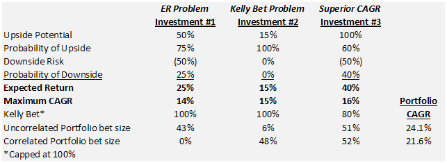
Correlation in Trial #1. But then I thought about the Central Limit Theorem and I realized that diversification makes a difference when assets are uncorrelated. But what if they are correlated? The benefit surely must be reduced. I subsequently built a string of payoffs where the gains and losses of Investment #1 and #3 occur in the same period (#2 doesn't matter because it always goes up 15%). When I recalculated the Correlated Portfolio position sizes, I got 0%, 48%, 52%. No exposure to Investment #1 in the Correlated Portfolio when the Uncorrelated Portfolio suggested a 43% position size.

This tells me that the correlation inside the array of outcomes has a large bearing on position size. What I needed to do is ensure that each array properly matches the intercorrelation amongst assets in the portfolio. At this point, I'm still working on that issue but maybe a starting point is the historical correlation and beta of each asset to the portfolio and other assets. Next, build thousands of hypothetical arrays of returns for each asset based on the scenario analysis. Finally, pick the set of hypothetical arrays that is most closely aligned with the inter-correlation of assets. From there we can iterate position sizes or use an optimization function that finds the portfolio with the maximum CAGR.

Speaking of maximum CAGR, see how both portfolios have higher Portfolio CAGR (24.1% and 21.6%) than any of the individual investments (14%, 15%, 16%)? This is the benefit of portfolio construction, which in this case is 5 to 10% of return.

Trial #2. The performance improvement of the portfolio made me wonder how a group of investments with similar Expected Returns (all 20%) but different payoff structures would look (see below).
‍

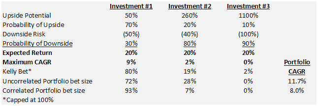
Here we see that neither the Uncorrelated or Correlated portfolio includes Investment #3 because it is severely impacted by its 90% chance of complete loss even though its expected return is 20% like the others. Investment #1 is favored by a wide margin because it has the lowest probability adjusted chance for loss of 15% (50% loss * 30% probability) versus 32% for Investment #2 (40% loss * 80% probability) versus 90% for Investment #3 (100% loss * 90% probability). In this case, the Kelly bet did a very good job of constructing the portfolio. This makes sense because the problem with the Kelly Formula for portfolio management is that it looks at each bet individually. We allowed the Kelly Formula to work individually by making all of the investments have the same Expected Return of 20%.

One of the most interesting outcomes of the second portfolio trial is that the CAGR of the Correlated Portfolio is 8.0%. That is lower than the 9% attained we could get from just betting the Kelly Bet of 80% in Investment #1 and holding the other 20% in cash. In this case, the best result is not a portfolio. I believe this is an important caveat in portfolio construction and should make cash an option for any portfolio. So instead of 3 Investments, you would always have 4 because cash may be a better option in certain circumstances.

Lessons Learned. So what have we learned from this analysis:

1) Kelly bet size alone is not sufficient to determine position size

2) Expected Return alone is not sufficient to determine position size

3) Investment correlation has a large bearing on position size

4) Probability Adjusted Chance for Loss has a large bearing on position size (Probability * Potential Loss)

5) Cash is a legitimate option even if it has a 0% expected return

Ultimate Solution. The ultimate solution requires incorporation of research's scenarios analysis, correlation amongst assets, and picking the array of position sizes that maximizes long-term geometric expected return. The first step is to forecast thousands of arrays of returns for each investment based on its probability weighted scenario analysis resulting from your analyst's research. Next, choose the one set of arrays from the thousands generated which most closely matches the correlation statistics for each asset and the portfolio. Finally, use the best set of arrays to interpolate the bet size for each investment that maximizes portfolio return (if someone knows of a closed-form way of producing the array of position sizes please let me know).

Problems with the Ultimate Solution.

1) Forecasting payout streams that have inter-correlation is very difficult. They could be calculated with historical correlations but that would suggest that future correlations will be the same as the past. The firm could forecast correlations but that is complicated and may be too much to ask from an operational perspective.

2) The arrays are constructed at random which causes them to change with each iteration. This could cause unnerving degrees of variance in optimal position sizes depending on the randomized set of arrays. For instance, you could see that the optimal position size for IBM is 4.3% one minute, have nothing change, and the optimal position size move to 4.6% because the random array being selected has changed. My guess is the arrays would have to be stabilized until the addition of a new asset or research is updated. There is some work being performed by Sam Savage to standardize arrays.

3) An optimization function is required to incorporate time horizon, liquidity, gross and net exposure, sector exposure, analysis confidence, etc. Certainly not an insurmountable hurdle, but could pose pitfalls.

Conclusion. Alpha Theory has tackled the problem in a straightforward way that accomplishes much of the task of position sizing described above. As we showed in Trial #1, Expected Return is a good predictor of position size in situations where there is variance in Expected Return. The predictive power is greatly enhanced by adjusting for the probability-weighted chance for loss (loss * probability of loss) which Alpha Theory does. The result is position sizing that is close to optimal position sizing (non-correlated). Lastly, because Alpha Theory is a linear function, it gives stable results and can scale position size to control for minimum and maximum position size, return parameters, liquidity, market correlation, time horizon, sector exposure, portfolio exposure, etc. Alpha Theory represents the best solution by providing most of the benefits of the complex ideal while still maintaining practicality for everyday use. At a bare minimum, it is light-years ahead of what most money managers are doing today!